
The dataset we are going to be using is coming from the UC Irvine Machine Learning Repository. This dataset contains approximately 76 features but for the classification problem we will be dealing with we will only be using 14 of them. Examples of these features would include: (age, sex, chol: serum cholestoral in mg/dl, and thalach: maximum heart rate achieved). A full list of the features being used can be seen within the Kaggle dataset description.
Here is the link to the Kaggle dataset:
https://www.kaggle.com/datasets/sumaiyatasmeem/heart-disease-classification-dataset.
If you want to follow along you can download the dataset from either of the two links provided above and import it into your notebook using pandas.
df = pd.read_csv("heart-disease.csv")
Exploring the Data
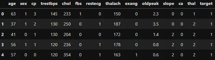
Lets see what our data looks like using df.head().
 using
using df.head()
df.shape #(rows, columns)
>(303, 14)
You can see above that their are 303 rows and 14 columns. This makes sense as we said above we are only using 14 features for our model development. And we also have 303 rows worth of data. Below is an image showing how balanced the dataset is, with 165 rows of data that are classed as having heart disease (1) and 138 classed as not having heart disease (0). Based on this initial analysis we can say that it’s a balanced dataset.
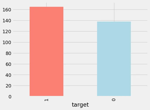 Image of the dataset targets.
Checking for Null Values
Checking for null values when training a model is important because most algorithms cannot handle missing or null values. Before going any further with Exploratory Data Analysis (EDA) it’s important to know what features have missing values and how much of it can you fill in and fix without removing too much of the data.
df.isna().sum()
age         0
sex         0
cp          0
trestbps    0
chol        0
fbs         0
restecg     0
thalach     0
exang       0
oldpeak     0
slope       0
ca          0
thal        0
target      0
dtype: int64
Using Pandas build in .isna() on the DataFrame and summing up the values with .sum() it will give us a breakdown of each of our features on missing values, NaN, and null values. In our case we don’t have any missing values which makes our life much easier as now we can carry on with the analysis.
What a machine learning algorithm really does is it looks for patterns in the data and compares them to the target variables. In our case our targets are going to be either a 1 for heart disease or a 0 for not heart disease. The algorithm will look at the 14 features we have and see what it can figure out in why a target is a 1 or 0. With enough data the machine learning algorithm will have learnt enough patterns in the data that it can make good predictions on new data it hasn’t seen before. This is what training is all about, having the algorithm learn enough patterns in the data to make good predictions. Lets see if we can figure out one of these patterns on our own based on the data we have.
One way to do this is by comparing our training features (we have 14) to the target variables and seeing the frequency of them.
df.sex.value_counts()
sex
1    207
0     96
Name: count, dtype: int64
We can see here that their are much more males that females, how do we know 1 are males and 0 are females? if you look at the dataset source at Kaggle & UC Irvine Machine Learning Repository it will tell you more information about the features. We can also use a pandas function called crosstab() to compare targets to the sex.
# Compare target columns with sex columne
pd.crosstab(df.target, df.sex)
sex 0 1
target
0 24 114
1 72 93
Using the crosstab function, we observe that within the ‘sex’ feature, Females (sex = 0) comprise 24 individuals without heart disease and 72 with heart disease. This shows a significant difference, approximately three times as many females have heart disease compared to those who do not. Machine learning algorithms can leverage these type of patterns. Based solely on this analysis, one might infer that for a new individual, if they are female, there is a likelihood of about 75% that they have heart disease. However, this inference is based solely on our current dataset; real-world data might vary.
Lets look at another example, we are going to look at the “cp” feature which is chest pain.
“cp” — chest pain type
- 0: Typical angina: chest pain related decrease blood supply to the heart
- 1: Atypical angina: chest pain not related to heart
- 2: Non-anginal pain: typically esophageal spasms (non heart related)
- 3: Asymptomatic: chest pain not showing signs of disease
Does chest pain relate to whether or not someone has heart disease? Lets find out.
# This will give you the output needed
pd.crosstab(df.cp, df.target)

# Make the crosstab more visual
pd.crosstab(df.cp, df.target).plot(kind="bar",
                                   figsize=(10,6),
                                   color=["salmon", "lightblue"])
plt.title("Heart Disease Frequency Per Chest Pain Type")
plt.xlabel("Chest Pain Type")
plt.ylabel("Amount")
plt.legend(["No Disease", "Disease"])
plt.xticks(rotation=0);
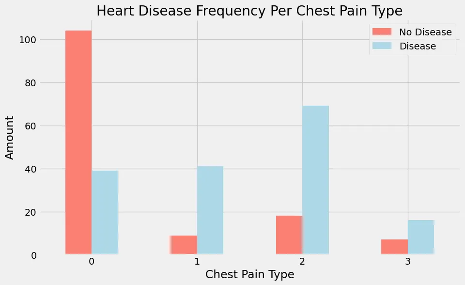 Heart Disease Frequency Per Chest Pain Type
Looking at the visual graph above that I created in jupyter with the code snippet above, you can see that if someone reports chest pain of 0 the majority are reported to not have heart disease (target = 0). Compare that now to people who report to have chest pain of 1 or 2, The majority of these patients are reported to have heart disease (target = 1).
Correlation between the independent variables are dependent variables
# Lets make our correlation matrix more visual
corr_matrix = df.corr()
fig, ax = plt.subplots(figsize=(15, 10))
ax = sns.heatmap(corr_matrix,
                annot=True,
                linewidths=0.5,
                fmt=".2f",
                cmap="YlGnBu");
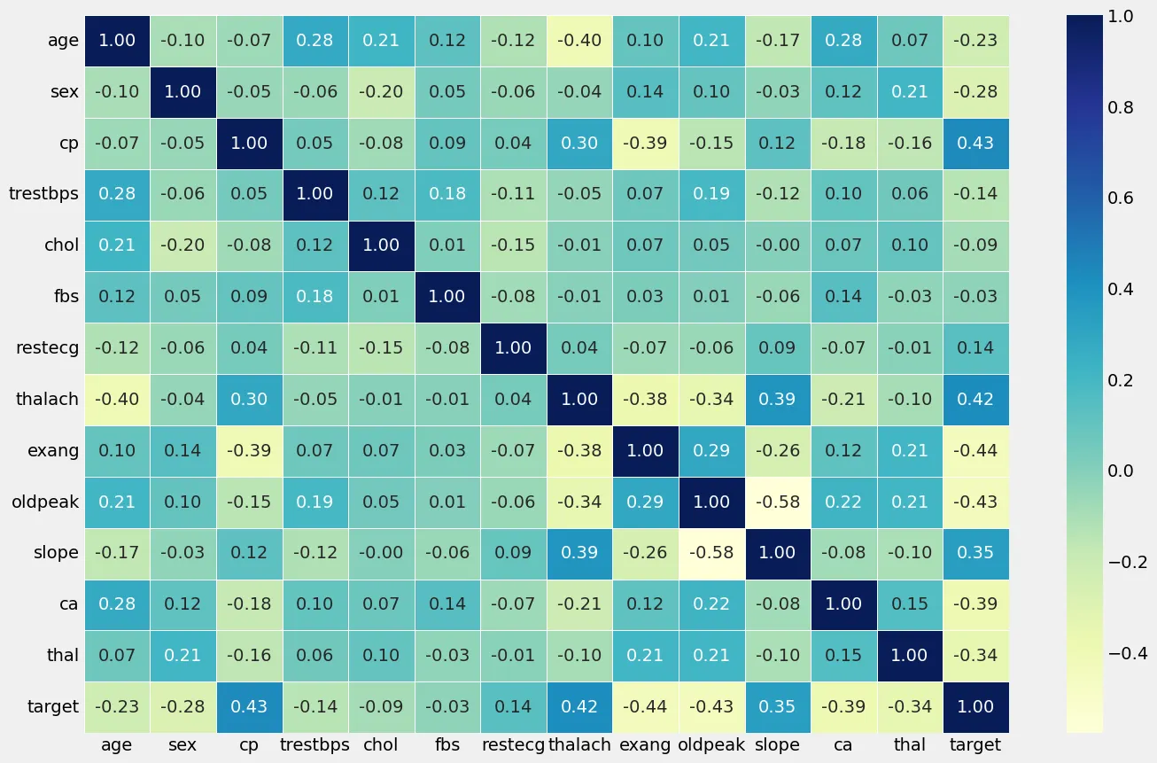 Correlation Matrix of independent & dependent features
Analyzing the correlation matrix between cp (chest pain type) and exang (exercise induced angina). The correlation matrix revealed a moderate positive correlation of 0.43 between cp and the presence of heart disease. This suggests that as the type of chest pain (cp) becomes more indicative of typical angina symptoms, there is a moderate tendency for the likelihood of heart disease to increase. Secondly, we can observed a moderate negative correlation of -0.44 between exang and heart disease presence. This implies that as the occurrence of exercise induced angina (exang) decreases, indicating a lower likelihood of angina during physical exertion, there is a moderate tendency for heart disease presence to increase. These findings underscore the potential predictive value of these features in assessing the risk of heart disease, highlighting their roles as important factors in our model development.
Model Development
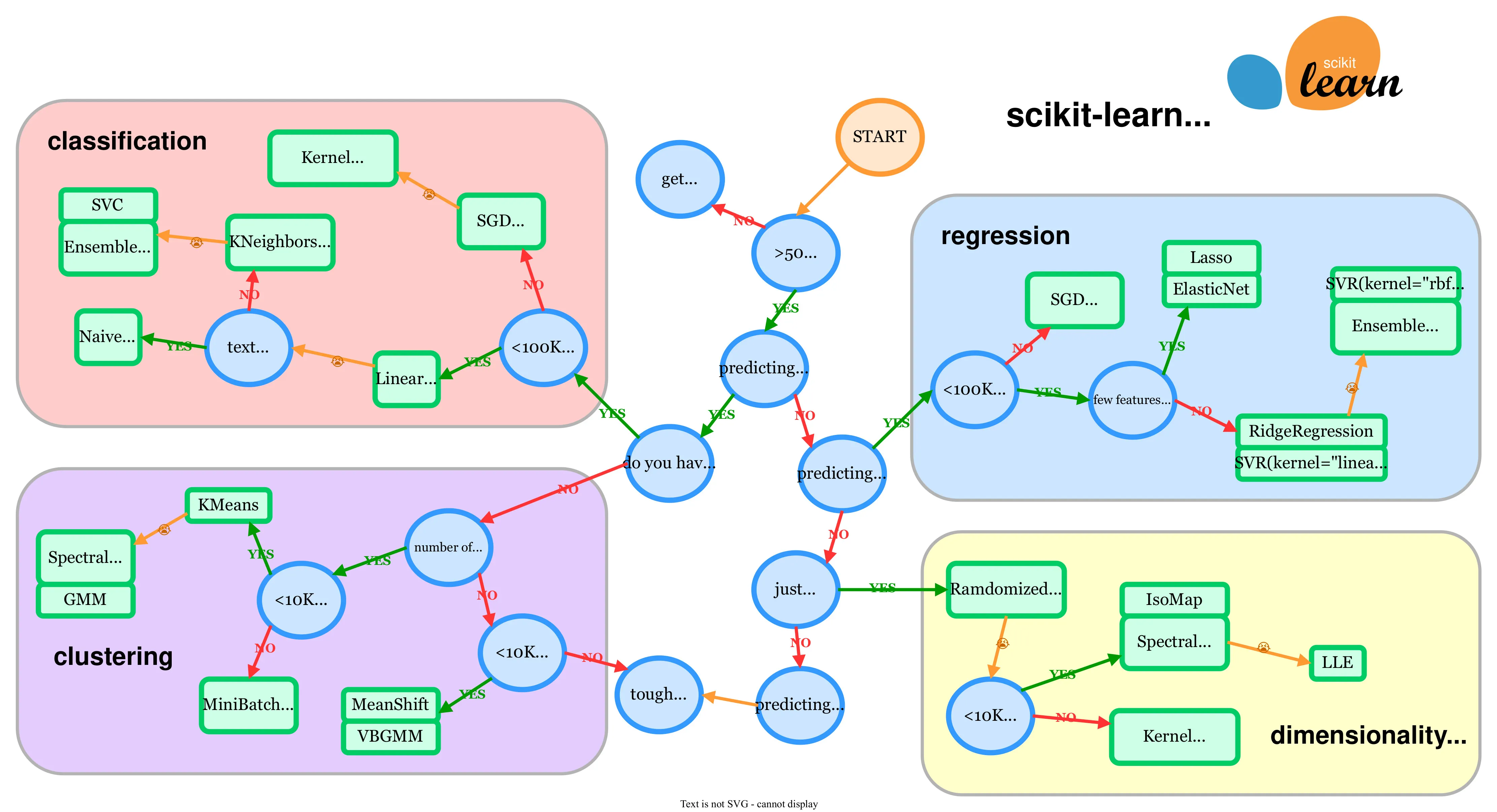 Scikit-learn choosing the right estimator image
The first thing you need to think about is what Machine Learning Algorithm are you going to use to train your model on? Scikit-learn has a handy webpage which shows a map just like the one above where it helps you in figuring out what algorithm to choose from. The green boxes are models you can pick from, and the blue circles are questions related to your problem. Our heart disease problem is a classification problem because we are prediction labels or classes 1 or 0, heart disease or not heart disease.
Before selecting and training our model for heart disease predictions, it is crucial to prepare our dataset appropriately. Our dataset consists of 14 features, which serve as our independent variables, and one target variable, which is the dependent variable indicating the presence of heart disease. To ensure that our model can generalize well to new data, we need to split our dataset into training and testing subsets. The training subset is used to train the model, while the testing subset is used to evaluate the model’s performance. In Python, the train_test_split() function from the scikit-learn library simplifies this process. We start by separating our features and target variable: x contains all features except the target, and y contains only the target variable. By setting a random seed with np.random.seed(42), we ensure the results are reproducible. We then use train_test_split(x, y, test_size=0.2), where x and y are our features and target variable respectively, and test_size=0.2 indicates that 20% of the data will be allocated to the testing set.
# Split the data into X & Y
x = df.drop("target", axis=1)
y = df["target"]

# Split data into train and test sets
np.random.seed(42)

# Split
x_train, x_test, y_train, y_test = train_test_split(x, y, test_size
We’re going to try 3 different machine learning models:
- Logistic Regression
- K-Nearest Neighbors Classifier
- Random Forest Classifier Lets create an easy function to train, fit, and evaluate our three models in one go instead of typing out all the Python code needed doing it manually.
# Put models in a dictionary
models = {"Logistic Regression": LogisticRegression(),
          "KNN": KNeighborsClassifier(),
          "Random Forest": RandomForestClassifier()}

# Create a function to fit and score models
def fit_and_score(models, X_train, X_test, y_train, y_test):
    """
    Fits and evaluates given machine learning models.
    models : a dict of differetn Scikit-Learn machine learning models
    X_train : training data (no labels)
    X_test : testing data (no labels)
    y_train : training labels
    y_test : test labels
    """
    # Set random seed
    np.random.seed(42)
    # Make a dictionary to keep model scores
    model_scores = {}
    # Loop through models
    for name, model in models.items():
        # Fit the model to the data
        model.fit(X_train, y_train)
        # Evaluate the model and append its score to model_scores
        model_scores[name] = model.score(X_test, y_test)
    return model_score
Now all we need to do is call fit_and_score() and pass it the models dictionary along with the x_train, x_test, y_train, y_test variables we got previously.
{'Logistic Regression': 0.8852459016393442,
 'KNN': 0.6885245901639344,
 'Random Forest': 0.8360655737704918}
This is how our models performed on our test data set. We now have baseline models, the best being the Logistic Regression algorithm with an accuracy of 88.5%. This is without tuning any of the hyperparameters. Hyperparameters are configurable settings that influence the training process and performance of machine learning algorithms. Tuning these hyperparameters can significantly enhance model performance. For example, adjusting the number of neighbors in KNN or the depth of trees in Random Forest can lead to better accuracy and generalization.
Hyperparameter Tuning
I’m going to give an example of tuning one of our models. In this example I’m going to pick the worst performing baseline model which is the KNN model with a baseline accuracy of 68.8%. Look at the Scikit-learn documentation on the K-Nearest Neighbors Classifier I can see one of the first changeable parameters is n_neighbors, and the default value is 5. This means that when we trained and scored our baseline KNN it used the default n_neighbors value of 5 as we didn’t change it. What would happen if we did change this value? tested the results and changed it again? and so on? The following Python code will do just that:
# Tune KNN
train_scores = []
test_scores = []

# Create a list of different values for n_neighbors
neighbors = range(1, 21)

# Setup KNN instance
knn = KNeighborsClassifier()

# loop through different n_neighbors
for i in neighbors:
    knn.set_params(n_neighbors=i)

    # Fit the algorithm
    knn.fit(x_train, y_train)

    # Update the training score list
    train_scores.append(knn.score(x_train, y_train))

    # Update the test score list
    test_scores.append(knn.score(x_test, y_test))
We are setting the n_neighbors value starting from 1 and ending at 21, and at the end of each interval we test the performance against the test data set for the models accuracy. I will then plot the results in an easy to read graph. Running the above code snipped will populate the train_scores &
test_scores arrays with the accuracy scores for each interval of the for loop. And finally plotting the results on a graph you can quickly see the performance overtime of the train accuracy and test accuracy. The Maximum KNN score on the test data was 75.41% as seen in the graph with the n_neighbors parameter set to 11. The default was 5 with a corresponding accuracy of 68.8%.
plt.plot(neighbors, train_scores, label="Train score")
plt.plot(neighbors, test_scores, label="Test score")
plt.xticks(np.arange(1,21, 1))
plt.xlabel("Number of n_neighbors")
plt.ylabel("Model score")
plt.legend()

print(f"Maxium KNN score on the test data: {max(test_scores)*100:.2f}%")
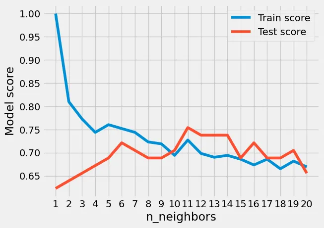 Hyperparameter Tuning of the KNN algorithm
We can see though that even with tuning the best accuracy we got with KNN was 75.41% which is still lower than the other baseline models without hyperparameter tuning. We will now see what accuracy we can get with tuning the other two models, using a different approach compared with the one we just did by hand, this time we will be using RandomizedSearchCV.
RandomizedSearchCV is a function in scikit-learn that helps automate the process of hyperparameter tuning. Unlike a traditional grid search, which exhaustively tries all combinations of parameters, RandomizedSearchCV selects a fixed number of parameter settings from a specified parameter grid. This random selection process allows it to explore a wider range of hyperparameters in less time, making it more efficient, especially when dealing with large datasets or complex models. Here are our hyperparameter grids for both the LogisticRegression and RandomForestClassifier models.
# Create a hyperparameter grid for LogisticRegression
log_reg_grid = {"C": np.logspace(-4, 4, 20),
                "solver": ["liblinear"]}

# Create a hyperparameter grid for RandomForestClassifier
rf_grid = {"n_estimators": np.arange(10, 1000, 50),
           "max_depth": [None, 3, 5, 10],
           "min_samples_split": np.arange(2, 20, 2),
           "min_samples_leaf": np.arange(1, 20, 2)}
We will now train our LogisticRegression model using RandomizedSearchCV to find the best hyperparameters from the grid we created above. Do keep in mind that not all possible hyperparameters will be checked here, RandomizedSearchCV will randomly pick from the grid we made and train and test the model with the hyperparameters it randomly picked. RandomizedSearchCV will do this based on how many iterations you choose from the n_iter parameter you pass it, in my case n_iter=20. This means RandomizedSearchCV will train and evaluate 20 different models with randomly picked hyperparameters from the hyperparameter grid for LogisticRegression above.
# Tune LogisticRegression

np.random.seed(42)

# Setup random hyperparameter search for LogisticRegression
rs_log_reg = RandomizedSearchCV(LogisticRegression(),
                                param_distributions=log_reg_grid,
                                cv=5,
                                n_iter=20,
                                verbose=True)

# Fit random hyperparameter search model for LogisticRegression
rs_log_reg.fit(x_train, y_train)
rs_log_reg.best_params_
The best hyperparameters it found were: {‘solver’: ‘liblinear’, ‘C’: 0.23357214690901212}. The accuracy using these hyperparameters remined the same which goes to show you how good LogisticRegression is at finding patterns in the data.
Next we are going to do the same for our RandomForestClassifier model.
# Setup random seed
np.random.seed(42)

# Setup random hyperparameter search for RandomForestClassifier
rs_rf = RandomizedSearchCV(RandomForestClassifier(),
                           param_distributions=rf_grid,
                           cv=5,
                           n_iter=20,
                           verbose=True)

# Fit random hyperparameter search model for RandomForestClassifier()
rs_rf.fit(x_train, y_train)
rs_rf.best_params_
# Evaluate the randomized search RandomForestClassifier model
rs_rf.score(x_test, y_test)
’’’ 0.8688524590163934 ‘’’
The best hyperparameters it found were: {‘n_estimators’: 210, ‘min_samples_split’: 4,‘min_samples_leaf’: 19,‘max_depth’: 3} The accuracy improved using these hyperparameters to 86.8% compared to the baseline of 83.6%.
Following our hyperparameter tuning with RandomizedSearchCV, the Logistic Regression model emerged as the top performer. To further refine this model, we will now utilize GridSearchCV to identify the optimal hyperparameters. Unlike RandomizedSearchCV, which randomly samples from a specified range of hyperparameters, GridSearchCV performs an exhaustive search across all possible combinations of the provided grid. This comprehensive approach ensures that every potential hyperparameter setting is evaluated, maximizing the chances of finding the best configuration.
# Different hyperparameters for our LogisticRegression model
log_reg_grid = {"C": np.logspace(-4, 4, 30),
                "solver": ["liblinear"]}

# Setup grid hyperparameter search for LogisticRegression
gs_log_reg = GridSearchCV(LogisticRegression(),
                          param_grid=log_reg_grid,
                          cv=5,
                          verbose=True)

# Fit grid hyperparameter search model
gs_log_reg.fit(x_train, y_train);
# Check the best hyperparmaters
gs_log_reg.best_params_
# Evaluate the grid search LogisticRegression model
gs_log_reg.score(x_test, y_test)
0.8852459016393442
The best hyperparameters it found were: {‘C’: 0.20433597178569418, ‘solver’: ‘liblinear’} yet the accuracy stayed the same at 88.5%. We could provide more hyperparameters within our grid for the LogisticRegression model and it could improve accuracy a bit more but at this stage we are going to finish up on hyperparameter tuning and improving the models and move onto evaluation and metrics.
Final Model Evaluation
We will use some different evaluation metrics that Scikit-learn provides. These metrics are only for classification models and not regression models. Sometimes you need more information than just the models accuracy.
Receiver Operating Characteristic (ROC):
# Make predictions with tuned model
y_preds = gs_log_reg.predict(x_test)
# Plot ROC curve and calculate and calculate AUC metric
from sklearn.metrics import roc_auc_score
roc_display = RocCurveDisplay.from_estimator(gs_log_reg, x_test, y_test)
plt.title(f"ROC Curve (AUC = {roc_auc_score(y_test, gs_log_reg.predict_proba(x_test)[:, 1]):.2f})")
plt.show()
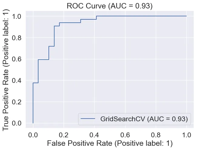 ROC Curve & AUC of 0.93
Area Under Curve (The ROC curve):
We achieved an AUC of 0.93 which is quite good as a perfect model will get 1.0.
Confusion Matrix:
 Import Seaborn
import seaborn as sns
sns.set(font_scale=1.5) # Increase font size

def plot_conf_mat(y_test, y_preds):
    """
    Plots a confusion matrix using Seaborn's heatmap().
    """
    fig, ax = plt.subplots(figsize=(3, 3))
    ax = sns.heatmap(confusion_matrix(y_test, y_preds),
                     annot=True, # Annotate the boxes
                     cbar=False,
                     cmap='viridis')
    plt.xlabel("Predicted label") # predictions go on the x-axis
    plt.ylabel("True label") # true labels go on the y-axis
    plt.title("Confusion Matrix")

plot_conf_mat(y_test, y_preds)
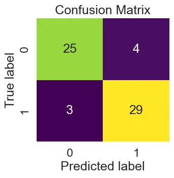 The Confusion Matrix
This shows the True Positive(TP), False Positive(FP), True Negative(TN), False Negative(FN) of our predictions using the LogisticRegression GridSearchCV model.
Classification Report:
print(classification_report(y_test, y_preds))
               precision    recall  f1-score   support

           0       0.89      0.86      0.88        29
           1       0.88      0.91      0.89        32

    accuracy                           0.89        61
   macro avg       0.89      0.88      0.88        61
weighted avg       0.89      0.89      0.89        61
And that finishes up the model evaluation for the Heart Disease model development. You could continue on and do even more evaluation metrics but it all depends on what your after and how much detail you need.